Ditsmod is a Node.js-based web framework designed for building highly extensible and fast applications. Another backend JavaScript framework, you say? Well, yes, but what options do we have as we enter 2025 in this stack? Probably 80% of all these frameworks suggest writing routes and middleware in the ExpressJS style. They look very concise when showcasing a “Hello, World!” example, but as soon as you move to even moderately sized projects (like RealWorld), it becomes a real challenge for the developer. This is one reason why microservices are so popular among these frameworks. Microservices are small, they don’t need to organize a lot of code.
But, in today’s context, there is already a more modern approach than ExpressJS like frameworks. TypeScript allows you to work not only with a much larger volume of code, it also provides completely new convenient possibilities for working with the IDE, with Dependency Injection.
So, why not just take for example the innovative NestJS and adapt it to your needs? The issue lies in the fact that NestJS has significant architectural flaws. However, its creator has already written a substantial amount of code for the framework’s ecosystem, so making architectural changes could result in breaking changes—something undesirable, especially given the solid user base of NestJS. For context, NestJS hit its first million weekly downloads in 2021, about 4.5 years after the initial commit. By the end of 2024, NestJS was being downloaded 4 million times a week. In my opinion, this statistic reflects an impressive growth rate for NestJS’s user base. At the same time, this rapid growth now hinders architectural changes because the creator is reluctant to risk losing users, often rejecting anything that could introduce breaking changes. For example, the transition to the ESM standard is not planned anytime soon for this very reason.
Ditsmod began development in 2020, also inspired by Angular v2+. I literally extracted Angular’s Dependency Injection module v4.4.7, which became the backbone of the future Ditsmod framework.
For those unfamiliar with Angular, I will try to explain the basic DI concepts borrowed from this framework in a simplified manner. Let’s consider the following example:
This example shows the Service3 class, which has two parameters in the constructor. The TypeScript compiler can transfer to the JavaScript code the information that the first place in the constructor of this class is Service1, and the second place is Service2. For this, you need to use the injectable decorator:
The mere fact that we can retrieve information about parameters defined in TypeScript code while working in JavaScript elevates the process of creating an instance of Service3 to a new level. This capability allows us to programmatically “understand” what Service3 requires in its constructor and automatically inject instances of the exact classes it needs.
It’s not necessary to work directly with the reflector to get familiar with Ditsmod, as most of its functionality works under the hood. You simply specify the required dependencies in the constructors of your classes, and Ditsmod automatically uses the reflector to determine what each class requires.
Returning to the comparison with other frameworks, it can be stated that the feature described above is likely unavailable in approximately 80% of all backend frameworks based on JavaScript or TypeScript. While the remaining frameworks do offer Dependency Injection (DI), they do not provide the same level of extensibility, modularity, and encapsulation as Ditsmod.
Up until version 3.0.0, Ditsmod had a small user base, which allowed for numerous breaking changes that introduced essential architectural improvements. Today, Ditsmod is a mature and stable framework. Starting with version 3.0.0, it adopted synchronized package versions, ensuring that any change to a package results in all packages being published with the same new version. Additionally, the entire Ditsmod codebase is written in the ESM format.
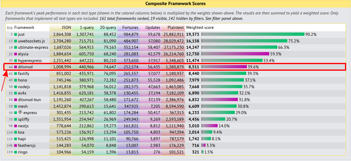
On the techempower website, you can view benchmarks for backend frameworks on the JavaScript stack. As you can see, according to the composite score, Ditsmod is the fastest framework that works on the basis of Node.js. Above it are only those frameworks that work on other JavaScript runtimes (Bun, Just-JS, uwebsockets).
About the repo
This monorepository uses yarn workspaces (see package.json).
During you run the following command:
corepack enable
corepack install
yarn install
cd packages/openapi
yarn build-ui
yarn will create symlinks in node_modules for all packages listed in the packages/* and examples/* folders. Also, modules in the packages/* folder are linked to the applications in the examples/* folder thanks to compilerOptions.paths as well as Project References. So, after any change in the source files in packages/*, these changes are automatically reflected in examples/*.
Development mode for any application in the examples/* directory can be started with this command:
This code repository is based on our arXiv tech report. Please read it for more information.
Deep neural networks are prone to adversarial examples that maliciously alter the network’s outcome. Due to the increasing popularity of 3D sensors in safety-critical systems and the vast deployment of deep learning models for 3D point sets, there is a growing interest in adversarial attacks and defenses for such models. So far, the research has focused on the semantic level, namely, deep point cloud classifiers. However, point clouds are also widely used in a geometric-related form that includes encoding and reconstructing the geometry.
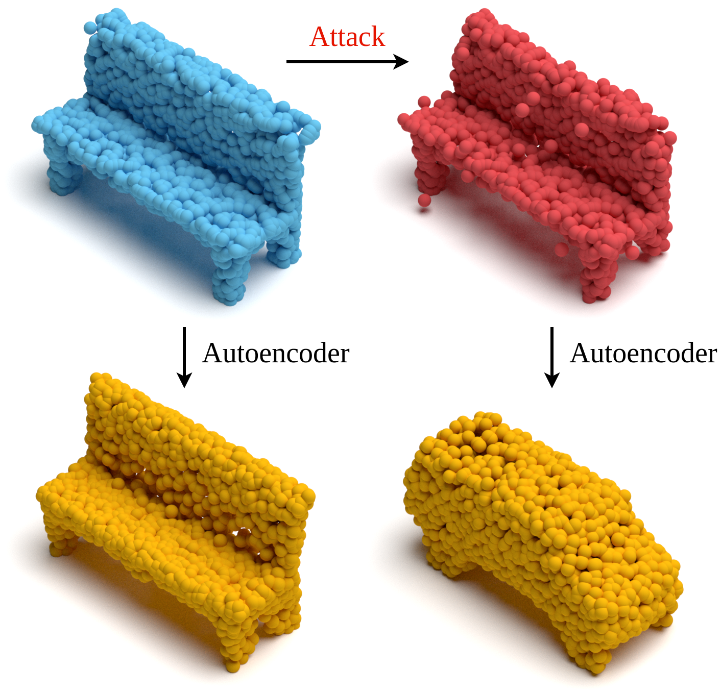
In this work, we are the first to consider the problem of adversarial examples at a geometric level. In this setting, the question is how to craft a small change to a clean source point cloud that leads, after passing through an autoencoder model, to the reconstruction of a different target shape. Our attack is in sharp contrast to existing semantic attacks on 3D point clouds. While such works aim to modify the predicted label by a classifier, we alter the entire reconstructed geometry. Additionally, we demonstrate the robustness of our attack in the case of defense, where we show that remnant characteristics of the target shape are still present at the output after applying the defense to the adversarial input.
Citation
If you find our work useful in your research, please consider citing:
@InProceedings{lang2021geometric_adv,
  author = {Lang, Itai and Kotlicki, Uriel and Avidan, Shai},
  title = {{Geometric Adversarial Attacks and Defenses on 3D Point Clouds}},
  booktitle = {Proceedings of the International Conference on 3D Vision (3DV)},
  pages = {1196--1205},
  year = {2021}
}
Installation
The code has been tested with Python 3.6.12, TensorFlow 1.13.2, TFLearn 0.3.2, PyTorch 1.6.0, CUDA 10.1, and cuDNN 7.6.5 on Ubuntu 16.04.
Compile TensorFlow ops: nearest neighbor grouping, implemented by Qi et al., and structural losses, implemented by Fan et al. The ops are located under external folder, in grouping and structural losses folders, respectively. The compilation scripts uses CUDA 10.1 path. If needed, modify the corresponding sh file of each op to point to your CUDA path. Then, use:
cd geometric_adv
sh compile_ops_tf.sh
An o and so files should be created in the corresponding folder of each op.
Compile PyTorch op: Chamfer Distance, implemented by Groueix et al. The op is located under transfer/atlasnet/auxiliary/ChamferDistancePytorch/chamfer3D folder. The following sh compilation script uses CUDA 10.1 path. If needed, modify script to point to your CUDA path. Then, use:
cd geometric_adv
sh compile_op_pt.sh
The compilation results should be created under transfer/atlasnet/build folder.
Usage
Overview
Our code is organized in the following folders:
autoencoder: scripts for training a victim autoencoder and an autoencoder for attack transfer.
classifier: source code for training a classifier for semantic interpretation, and scripts for semantic evaluation of the attacks and defenses.
transfer: source code for training an AtlasNet autoencoder and a FoldingNet autoencoder for attack transfer (under atlasnet and foldingnet folders, respectively), and scripts for running attack transfer.
src: implementation of the autoencoder for attack, the adversary, and utility helper functions.
external: external public source code, implementing TensorFlow ops and Python i/o for ply files.
The following sub-sections explain the following items:
Download Models and Data: how to download the trained models and data used for the experiments in our work.
Download the trained models and data for our experiments:
cd geometric_adv
bash download_models_and_data.sh
The models (about 200MB) will be saved under log folder, in the following folders:
autoencoder_victim: a victim autoencoder for the attack and defense experiments.
pointnet: a classifier for the semantic interpretation experiment.
autoencoder_for_transfer, atlasnet_for_transfer, and foldingnet_for_transfer: autoencoders for the attack transfer experiment.
The data (about 220MB) will be saved under log/autoencoder_victim/eval folder.
Attacks
First, save the default configuration of the victim autoencoder using:
cd autoencoder
python train_ae.py --train_folder log/autoencoder_victim --save_config_and_exit 1
The configuration will be saved to the folder log/autoencoder_victim.
Then, prepare indices for the attack using:
cd ../attacker
bash runner_indices_for_attack.sh
The script will prepare random indices for source point clouds to attack. It will also prepare a nearest neighbors matrix that will be used for selecting target point cloud candidates for the attack. The data will be saved to log/autoencoder_victim/eval folder.
Next, run and evaluate the output and latent space attacks using:
cd ../attacker
sh runner_attacker.sh
Attack results will be saved to the folders log/autoencoder_victim/eval/output_space_attack and log/autoencoder_victim/eval/latent_space_attack. Under the attack folder there is a folder for each source class.
The script runner_attacker.sh uses the following scripts:
run_attack.py is used to optimize the attack. For each source class folder, it saves adversarial metrics (adversarial_metrics.npy), adversarial examples (adversarial_pc_input.npy), and their reconstruction by the victim autoencoder (adversarial_pc_recon.npy).
get_dists_per_point.py computes additional data required for the attack evaluation (adversarial_pc_input_dists.npy).
evaluate_attack.py analyzes the attack results. Statistics for the attack will be saved to the file over_classes/eval_stats.txt.
When running evaluate_attack.py, you can use the following additional flags:
--save_graphs 1: to save graphs of adversarial metrics for each source class.
--save_pc_plots 1: to save visualization of the source point clouds, adversarial examples, target point clouds, and their reconstruction.
Defenses
Run critical points and off-surface defenses against the output and latent space attacks using:
cd ../defender
sh runner_defender.sh
Under each attack folder, defense results will be saved to the folders defense_critical_res and defense_surface_res. Under these defense folders, there is a folder for each source class.
The script runner_defender.sh uses the following scripts:
run_defense_critical.py and run_defense_surface.py save defense metrics (defense_metrics.npy), defended point clouds (defended_pc_input.npy), and their reconstruction by the victim autoencoder (defended_pc_recon.npy). These files will be saved to each source class folder.
evaluate_defense.py analyzes the defense results. Statistics for the defense will be saved to the file over_classes/eval_stats.txt.
When running evaluate_defense.py, you can use the following additional flags:
--save_graphs 1: to save graphs of defense metrics for each source class.
--save_pc_plots 1: to save visualization of the source point clouds, adversarial examples, defended point clouds, and their reconstructions. In the adversarial examples, points that are filtered by the defense will be marked in Red.
--use_adversarial_data 0: to evaluate the defense results on source point clouds.
Semantic Interpretation
Use the trained classifier to evaluate the semantic interpretation of reconstructed adversarial and defended point clouds:
cd ../classifier
sh runner_classifier.sh
The script runner_classifier.sh uses the following scripts:
run_classifier.py gets the classifier’s predictions for reconstructed adversarial and defended point clouds. The classifier’s results will be saved under the corresponding attack and defense folders to a folder named classifer_res. Under this folder, there is a folder for each source class with the classifier’s predictions.
evaluate_classifier.py evaluates the semantic interpretation of the reconstructed point clouds. Statistics for the classifier will be saved to the folder classifer_res/over_classes.
Note:
The semantic interpretation of reconstructed source and target point clouds is also evaluated (for reference). The name for the classifier’s folder, in this case, is classifer_res_orig.
When running evaluate_classifier.py, you can use an additional flag --save_graphs 1, to save graphs of the classifier’s predictions for each source class.
Transfer
Run and evaluate the adversarial examples through the autoencoders for attack transfer using:
cd ../transfer
sh runner_transfer.sh
This script will run the adversarial examples of the output and latent space attacks through the three autoencoders for transfer described above. If you trained part of these autoencoders, edit the script accordingly.
The script runner_transfer.sh uses the following scripts:
run_transfer.py uses an autoencoder for transfer to reconstruct adversarial point clouds (transferred_pc_recon.npy) and compute transfer metrics (transfer_metrics.npy) for each source class. The results are saved to an attack transfer folder, under the autoencoder for transfer. For instance: log/autoencoder_for_transfer/output_space_attack_transfer.
evaluate_transfer.py compute transfer statistics that are saved to the file over_classes/eval_stats.txt under the attack transfer folder.
When running evaluate_transfer.py, you can use the following additional flags:
--save_graphs 1: to save graphs of transfer metrics for each source class.
--save_pc_plots 1: to save visualization of the source point clouds, adversarial examples, and their reconstructions by the victim autoencoder or autoencoder for transfer.
Retrain Models
In the previous section you employed the models that we used in our work. In this section we explain the steps for retraining these models. It may be useful as a reference example, in case you want to use different data than that we used.
Each point cloud contains 2048 points, uniformly sampled from the shape surface. The data will be downloaded to a folder named geometric_adv/data/shape_net_core_uniform_samples_2048.
Victim Autoencoder
Train a victim autoencoder model using:
cd autoencoder
sh runner_ae_for_attack.sh
The model will be saved to the folder log/autoencoder_victim.
The script runner_ae_for_attack.sh uses the following scripts:
train_ae.py is used to train the autoencoder.
tst_ae.py prepares data for attack. The data will be saved to the folder log/autoencoder_victim/eval.
Classifier
First, prepare data for training a classifier for semantic interpretation using:
cd ../autoencoder
sh runner_ae_for_classifier.sh
This script saves the point clouds of the train and validation sets that were used during the victim autoencoder’s training. These points clouds and their labels will be used for training the classifier. The data will be saved to the folders log/autoencoder_victim/eval_train and log/autoencoder_victim/eval_val. Note that these point clouds of the train the validation sets will be used for the training of autoencoders for transfer (see seb-section Autoencoders for Attack Transfer below).
Then, train the classifier using:
cd ../classifier
python train_classifier.py
Autoencoders for Attack Transfer
Train autoencoders other than the victim one to perform attack transfer. These autoencoders will be trained on the same data set as the attacked autoencoder. Note that the autoencoders for transfer are independent of each other, and you can choose which one to train and run transfer with.
To train an autoencoder with the same architecture of the victim and different weight initialization, use:
cd ../autoencoder
sh runner_ae_for_transfer.sh
The model will be saved to the folder log/autoencoder_for_transfer.
To train an AtlasNet autoencoder, use:
cd ../transfer/atlasnet
sh runner_atlasnet.sh
The model will be saved to the folder log/atlasnet_for_transfer.
To train a FoldingNet autoencoder, use:
cd ../../transfer/foldingnet
sh runner_foldingnet.sh
The model will be saved to the folder log/foldingnet_for_transfer.
License
This project is licensed under the terms of the MIT license (see the LICENSE file for more details).
This code repository is based on our arXiv tech report. Please read it for more information.
Deep neural networks are prone to adversarial examples that maliciously alter the network’s outcome. Due to the increasing popularity of 3D sensors in safety-critical systems and the vast deployment of deep learning models for 3D point sets, there is a growing interest in adversarial attacks and defenses for such models. So far, the research has focused on the semantic level, namely, deep point cloud classifiers. However, point clouds are also widely used in a geometric-related form that includes encoding and reconstructing the geometry.
In this work, we are the first to consider the problem of adversarial examples at a geometric level. In this setting, the question is how to craft a small change to a clean source point cloud that leads, after passing through an autoencoder model, to the reconstruction of a different target shape. Our attack is in sharp contrast to existing semantic attacks on 3D point clouds. While such works aim to modify the predicted label by a classifier, we alter the entire reconstructed geometry. Additionally, we demonstrate the robustness of our attack in the case of defense, where we show that remnant characteristics of the target shape are still present at the output after applying the defense to the adversarial input.
Citation
If you find our work useful in your research, please consider citing:
@InProceedings{lang2021geometric_adv,
  author = {Lang, Itai and Kotlicki, Uriel and Avidan, Shai},
  title = {{Geometric Adversarial Attacks and Defenses on 3D Point Clouds}},
  booktitle = {Proceedings of the International Conference on 3D Vision (3DV)},
  pages = {1196--1205},
  year = {2021}
}
Installation
The code has been tested with Python 3.6.12, TensorFlow 1.13.2, TFLearn 0.3.2, PyTorch 1.6.0, CUDA 10.1, and cuDNN 7.6.5 on Ubuntu 16.04.
Compile TensorFlow ops: nearest neighbor grouping, implemented by Qi et al., and structural losses, implemented by Fan et al. The ops are located under external folder, in grouping and structural losses folders, respectively. The compilation scripts uses CUDA 10.1 path. If needed, modify the corresponding sh file of each op to point to your CUDA path. Then, use:
cd geometric_adv
sh compile_ops_tf.sh
An o and so files should be created in the corresponding folder of each op.
Compile PyTorch op: Chamfer Distance, implemented by Groueix et al. The op is located under transfer/atlasnet/auxiliary/ChamferDistancePytorch/chamfer3D folder. The following sh compilation script uses CUDA 10.1 path. If needed, modify script to point to your CUDA path. Then, use:
cd geometric_adv
sh compile_op_pt.sh
The compilation results should be created under transfer/atlasnet/build folder.
Usage
Overview
Our code is organized in the following folders:
autoencoder: scripts for training a victim autoencoder and an autoencoder for attack transfer.
classifier: source code for training a classifier for semantic interpretation, and scripts for semantic evaluation of the attacks and defenses.
transfer: source code for training an AtlasNet autoencoder and a FoldingNet autoencoder for attack transfer (under atlasnet and foldingnet folders, respectively), and scripts for running attack transfer.
src: implementation of the autoencoder for attack, the adversary, and utility helper functions.
external: external public source code, implementing TensorFlow ops and Python i/o for ply files.
The following sub-sections explain the following items:
Download Models and Data: how to download the trained models and data used for the experiments in our work.
Download the trained models and data for our experiments:
cd geometric_adv
bash download_models_and_data.sh
The models (about 200MB) will be saved under log folder, in the following folders:
autoencoder_victim: a victim autoencoder for the attack and defense experiments.
pointnet: a classifier for the semantic interpretation experiment.
autoencoder_for_transfer, atlasnet_for_transfer, and foldingnet_for_transfer: autoencoders for the attack transfer experiment.
The data (about 220MB) will be saved under log/autoencoder_victim/eval folder.
Attacks
First, save the default configuration of the victim autoencoder using:
cd autoencoder
python train_ae.py --train_folder log/autoencoder_victim --save_config_and_exit 1
The configuration will be saved to the folder log/autoencoder_victim.
Then, prepare indices for the attack using:
cd ../attacker
bash runner_indices_for_attack.sh
The script will prepare random indices for source point clouds to attack. It will also prepare a nearest neighbors matrix that will be used for selecting target point cloud candidates for the attack. The data will be saved to log/autoencoder_victim/eval folder.
Next, run and evaluate the output and latent space attacks using:
cd ../attacker
sh runner_attacker.sh
Attack results will be saved to the folders log/autoencoder_victim/eval/output_space_attack and log/autoencoder_victim/eval/latent_space_attack. Under the attack folder there is a folder for each source class.
The script runner_attacker.sh uses the following scripts:
run_attack.py is used to optimize the attack. For each source class folder, it saves adversarial metrics (adversarial_metrics.npy), adversarial examples (adversarial_pc_input.npy), and their reconstruction by the victim autoencoder (adversarial_pc_recon.npy).
get_dists_per_point.py computes additional data required for the attack evaluation (adversarial_pc_input_dists.npy).
evaluate_attack.py analyzes the attack results. Statistics for the attack will be saved to the file over_classes/eval_stats.txt.
When running evaluate_attack.py, you can use the following additional flags:
--save_graphs 1: to save graphs of adversarial metrics for each source class.
--save_pc_plots 1: to save visualization of the source point clouds, adversarial examples, target point clouds, and their reconstruction.
Defenses
Run critical points and off-surface defenses against the output and latent space attacks using:
cd ../defender
sh runner_defender.sh
Under each attack folder, defense results will be saved to the folders defense_critical_res and defense_surface_res. Under these defense folders, there is a folder for each source class.
The script runner_defender.sh uses the following scripts:
run_defense_critical.py and run_defense_surface.py save defense metrics (defense_metrics.npy), defended point clouds (defended_pc_input.npy), and their reconstruction by the victim autoencoder (defended_pc_recon.npy). These files will be saved to each source class folder.
evaluate_defense.py analyzes the defense results. Statistics for the defense will be saved to the file over_classes/eval_stats.txt.
When running evaluate_defense.py, you can use the following additional flags:
--save_graphs 1: to save graphs of defense metrics for each source class.
--save_pc_plots 1: to save visualization of the source point clouds, adversarial examples, defended point clouds, and their reconstructions. In the adversarial examples, points that are filtered by the defense will be marked in Red.
--use_adversarial_data 0: to evaluate the defense results on source point clouds.
Semantic Interpretation
Use the trained classifier to evaluate the semantic interpretation of reconstructed adversarial and defended point clouds:
cd ../classifier
sh runner_classifier.sh
The script runner_classifier.sh uses the following scripts:
run_classifier.py gets the classifier’s predictions for reconstructed adversarial and defended point clouds. The classifier’s results will be saved under the corresponding attack and defense folders to a folder named classifer_res. Under this folder, there is a folder for each source class with the classifier’s predictions.
evaluate_classifier.py evaluates the semantic interpretation of the reconstructed point clouds. Statistics for the classifier will be saved to the folder classifer_res/over_classes.
Note:
The semantic interpretation of reconstructed source and target point clouds is also evaluated (for reference). The name for the classifier’s folder, in this case, is classifer_res_orig.
When running evaluate_classifier.py, you can use an additional flag --save_graphs 1, to save graphs of the classifier’s predictions for each source class.
Transfer
Run and evaluate the adversarial examples through the autoencoders for attack transfer using:
cd ../transfer
sh runner_transfer.sh
This script will run the adversarial examples of the output and latent space attacks through the three autoencoders for transfer described above. If you trained part of these autoencoders, edit the script accordingly.
The script runner_transfer.sh uses the following scripts:
run_transfer.py uses an autoencoder for transfer to reconstruct adversarial point clouds (transferred_pc_recon.npy) and compute transfer metrics (transfer_metrics.npy) for each source class. The results are saved to an attack transfer folder, under the autoencoder for transfer. For instance: log/autoencoder_for_transfer/output_space_attack_transfer.
evaluate_transfer.py compute transfer statistics that are saved to the file over_classes/eval_stats.txt under the attack transfer folder.
When running evaluate_transfer.py, you can use the following additional flags:
--save_graphs 1: to save graphs of transfer metrics for each source class.
--save_pc_plots 1: to save visualization of the source point clouds, adversarial examples, and their reconstructions by the victim autoencoder or autoencoder for transfer.
Retrain Models
In the previous section you employed the models that we used in our work. In this section we explain the steps for retraining these models. It may be useful as a reference example, in case you want to use different data than that we used.
Each point cloud contains 2048 points, uniformly sampled from the shape surface. The data will be downloaded to a folder named geometric_adv/data/shape_net_core_uniform_samples_2048.
Victim Autoencoder
Train a victim autoencoder model using:
cd autoencoder
sh runner_ae_for_attack.sh
The model will be saved to the folder log/autoencoder_victim.
The script runner_ae_for_attack.sh uses the following scripts:
train_ae.py is used to train the autoencoder.
tst_ae.py prepares data for attack. The data will be saved to the folder log/autoencoder_victim/eval.
Classifier
First, prepare data for training a classifier for semantic interpretation using:
cd ../autoencoder
sh runner_ae_for_classifier.sh
This script saves the point clouds of the train and validation sets that were used during the victim autoencoder’s training. These points clouds and their labels will be used for training the classifier. The data will be saved to the folders log/autoencoder_victim/eval_train and log/autoencoder_victim/eval_val. Note that these point clouds of the train the validation sets will be used for the training of autoencoders for transfer (see seb-section Autoencoders for Attack Transfer below).
Then, train the classifier using:
cd ../classifier
python train_classifier.py
Autoencoders for Attack Transfer
Train autoencoders other than the victim one to perform attack transfer. These autoencoders will be trained on the same data set as the attacked autoencoder. Note that the autoencoders for transfer are independent of each other, and you can choose which one to train and run transfer with.
To train an autoencoder with the same architecture of the victim and different weight initialization, use:
cd ../autoencoder
sh runner_ae_for_transfer.sh
The model will be saved to the folder log/autoencoder_for_transfer.
To train an AtlasNet autoencoder, use:
cd ../transfer/atlasnet
sh runner_atlasnet.sh
The model will be saved to the folder log/atlasnet_for_transfer.
To train a FoldingNet autoencoder, use:
cd ../../transfer/foldingnet
sh runner_foldingnet.sh
The model will be saved to the folder log/foldingnet_for_transfer.
License
This project is licensed under the terms of the MIT license (see the LICENSE file for more details).
This Python script demonstrates how to automate posting a tweet on Twitter using the Selenium web automation library. It opens a Chrome web browser, logs into a Twitter account, composes a tweet, and posts it.
Prerequisites
Before running the script, make sure you have the following prerequisites installed:
Wait for a specified time (e.g., 60 seconds) to ensure the tweet is posted:
time.sleep(60)
Quit the Chrome driver:
driver.quit()
Customize the script to meet your specific automation needs, such as logging in with your Twitter account and posting the desired content.
Notes
This script logs into Twitter using an existing account’s session data. Make sure to replace os.getcwd() with the appropriate directory path if needed.
Be cautious while automating actions on websites to comply with their terms of service.
You can customize the script and README.md file further to suit your specific requirements and ensure you have the correct WebDriver for Chrome installed.
This repository aims to help code beginners with their first successful pull request and open source contribution. 🥳
⭐ Feel free to use this project to make your first contribution to an open-source project on GitHub. Practice making your first pull request to a public repository before doing the real thing!
⭐ Make sure to grab some cool swags during Hacktoberfest by getting involved in the open-source community.
This repository is open to all Members of the GitHub community.
Any member can contribute to this project! 😁
What is Hacktoberfest? 🤔
A month-long celebration from October 1st to October 31st presented by Digital Ocean and DEV Community collaborated with GitHub to get people involved in Open Source. Create your very first pull request to any public repository on GitHub and contribute to the open-source developer community.
To qualify for the official limited edition Hacktoberfest shirt, you must register here and make four Pull Requests (PRs) between October 1-31, 2022 (in any time zone). PRs can be made to any public repository on GitHub, not only the ones with issues labeled Hacktoberfest. This year, the first 40,000 participants who complete the challenge will earn a T-shirt.
Steps to follow 📜
Tip : Complete this process in GitHub (in your browser)
flowchart LR
    Fork[Fork the project]-->branch[Create a New Branch]
    branch-->Edit[Edit file]
    Edit-->commit[Commit the changes]
    commit -->|Finally|creatpr((Create a Pull Request))
Loading
To know how to contribute go through this page Contributor.md
still if you want help than create a issue and add your quiry
pyZDCF is a Python module that emulates a widely used Fortran program called ZDCF (Z-transformed Discrete Correlation Function, Alexander 1997). It is used for robust estimation of cross-correlation function of sparse and unevenly sampled astronomical time-series. This Python implementation also introduces sparse matrices in order to significantly reduce RAM usage when running the code on large time-series (> 3000 points).
pyZDCF is based on the original Fortran code fully developed by
Prof. Tal Alexander from Weizmann Institute of Science, Israel
(see Acknowledgements and References for details and further reading).
Development of pyZDCF module was motivated by the long and successful usage of
the original ZDCF Fortran code in the analysis of light curves of active galactic
nuclei by our research group (see Kovacevic et al. 2014, Shapovalova et al. 2019, and reference therein). One of the science cases we investigate is photometric reverberation mapping in the context of Legacy Survey of Space and Time (LSST) survey strategies (see Jankov et al. 2022). However, this module is general and is meant to be used for cross-correlation of spectroscopic or photometric light curves, same as the original Fortran version.
Older versions of pyzdcf support older versions of Python, see table for details:
pyzdcf Version
Supported Python Versions
Notes
>= 1.0.3
3.9 – 3.13
Requires newer dependencies (e.g. pandas ≥2.2.3)
<= 1.0.2
3.8 – 3.11
Compatible with older environments
How to use
Input files
This code requires user-provided plain text files as input. CSV files are
accepted by default, but you can use any other delimited file, as long as you
provide the sep keyword argument when calling pyzdcf function. The input
light curve file should be in 3 columns: time (ordered), flux/magnitude and
absolute error on flux/magnitude. Make sure to exclude the header (column
names) from the input files.
First few lines of the example input file accepted by default (CSV):
NOTE: pyZDCF is tested only with input files having whole numbers (integers) for time column. If you have decimal numbers (e.g., you have a light curve with several measurments in the same night expressed as fractions of a day instead of minutes), just convert them into a time format with integer values (e.g., minutes instead of days). On the other hand, you could round the values from the same day (e.g. 5.6 –> 5, 5.8 –> 5, etc.) and the algorithm will take in the information and average the flux for that day.
Input parameters
If you use interactive mode (intr = True), then pyZDCF will ask you to
enter all input parametars interactively, similarly to original ZDCF interface.
There is also a manual mode (intr = False) where you can provide input
parameters using a dictionary and passing it to parameters keyword argument.
Available input parameters (keys in the parameters dictionary) are:
autocf – if True, perform auto-correlation, otherwise do the cross-correlation.
prefix – provide a name for the output file.
uniform_sampling – if True, set flag to perform uniform sampling of the light curve.
omit_zero_lags – if True, omit zero lag points.
minpts – minimal number of points per bin.
num_MC – number of Monte Carlo simulations for error estimation.
lc1_name – Name of the first light curve file
lc2_name – Name of the second light curve file (required only if we do cross-correlation)
For more information on the correct syntax, see “Running the code” subsection.
Output
The return value of the pyzdcf function is a pandas.DataFrame object displaying the results in 7 columns:
The columns are: time-lag, negative time-lag std, positive time-lag std, zdcf,
negative zdcf sampling error, positive zdcf sampling error, number of points
per bin. For more information on how these values are calculated see
Alexander 1997.
The code will also generate an output .dcf file file in a specified folder on your computer with same 7 columns containing the results. It is allowed to name these files however you want using the prefix parameter (see example in the next subsection).
Optionally, by adding keyword argument savelc = True, pyzdcf can create and save light curve files used as input after averaging points with identical times.
Running the code
An example for calculating cross-correlation between two light curves:
frompyzdcfimportpyzdcfinput='./input/'# Path to the input dataoutput='./output/'# Path to the directory for saving the results# Light curve nameslc1='lc_name1'lc2='lc_name2'# Parameters are passed to the pyZDCF as a dictionaryparams=dict(autocf=False, # Autocorrelation (T) or cross-correlation (F)prefix='ccf', # Output files prefixuniform_sampling=False, # Uniform sampling?omit_zero_lags=True, # Omit zero lag points?minpts=0, # Min. num. of points per bin (0 is a flag for default value of 11)num_MC=100, # Num. of Monte Carlo simulations for error estimationlc1_name=lc1, # Name of the first light curve filelc2_name=lc2# Name of the second light curve file (required only if we do CCF)
)
# Here we use non-interactive mode (intr=False)dcf_df=pyzdcf(input_dir=input,
output_dir=output,
intr=False,
parameters=params,
sep=',',
sparse='auto',
verbose=True)
# To run the program in interactive mode (like the original Fortran code):dcf_df=pyzdcf(input_dir=input,
output_dir=output,
intr=True,
sep=',',
sparse='auto',
verbose=True
)
Additionally, you can also check out code description of the original Fortran version because the majority of input parameters and all output files are the same as in pyZDCF. You can download the fortran source code here.
Features
Sparse matrix implementation for reduced RAM usage when working with long light curves (>3000 points);
The main benefit is that we can now run these demanding calculations on our own personal computers (8 GB of RAM is enough for
light curves containing up to 15000 points), making the usage of this algorithm more convinient than ever.
You can turn this on/off by specifying sparse keyword argument to True or False. Default value is 'auto', where sparse marices are utilized when there are more than 3000 points per light curve. Note that by reducing RAM usage, we pay in increased program running time.
Interactive mode: program specifically asks the user to provide necessary parameters (similar to original Fortran version);
Manual mode: user can provide all parameters in one dictionary.
Fixed bugs from original ZDCF (v2.3) written in Fortran 95.
The module was tested (i.e., compared with original ZDCF v2.3 output, with fixed bugs) for various parameter combinations on a set of 100 AGN light curve candidates (g and r bands). The list of object ids and coordinates was taken from a combined catalogue of known AGNs (Sánchez-Sáez et al. 2021).
If you use pyZDCF for scientific work leading to a publication,
please consider acknowledging it using the following citation (BibTeX):
@software{jankov_isidora_2022_7253034,
  author       = {Jankov, Isidora and
                  Kovačević, Andjelka B. and
                  Ilić, Dragana and
                  Sánchez-Sáez, Paula and
                  Nikutta, Robert},
  title        = {pyZDCF: Initial Release},
  month        = oct,
  year         = 2022,
  publisher    = {Zenodo},
  version      = {v1.0.0},
  doi          = {10.5281/zenodo.7253034},
  url          = {https://doi.org/10.5281/zenodo.7253034}
}
The pyZDCF module is based on the original Fortran code developed by Prof. Tal Alexander (Weizmann Institute of Science, Israel). Download Fortran version from professor’s page.
For theoretical details regarding the ZDCF algorithm see this publication: Alexander, T. (1997).
Huge thanks to my closest collegues and mentors Dr. Andjelka Kovačević and Dr. Dragana Ilić, as well as to Dr. Paula Sánchez-Sáez and Dr. Robert Nikutta for invaluable input during the development and testing of this python module.
Many thanks to Prof. Eli Waxman, Amir Bar On and former students of Prof. Tal Alexander for their kind assistance regarding the development of pyZDCF module and its acknowledgment as part of the legacy behind late Prof. Alexander.
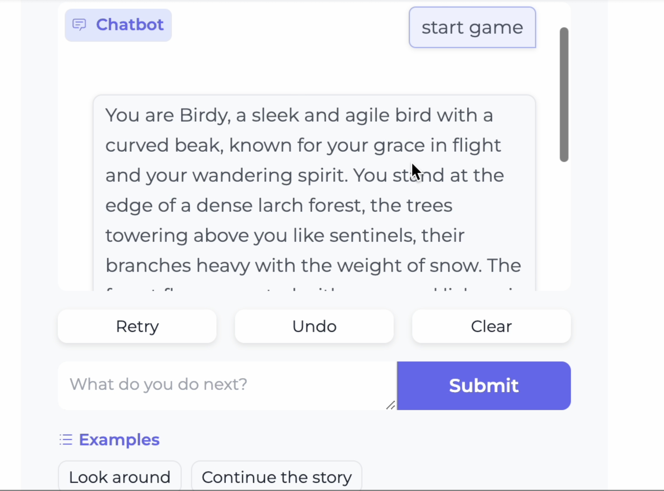
Birdy’s Journey: An AI-Powered Text Adventure Game
Read my Medium post where I explained development process, explain the code in detail, and share insights from this rapid 6-hour project!
An AI-powered text adventure where you step into the wings of Birdy, the last Slender-billed Curlew.
The Story
It all began with a tweet—a solemn announcement of the extinction of the Slender-billed Curlew (Numenius tenuirostris). The thought of the last of its kind soaring through a silent, unresponsive world struck a deep chord within me. I wanted to give life to this poignant narrative and allow others to experience it firsthand.
So, in just 6 hours, I crafted Birdy’s Journey, a text-based adventure game that immerses you in the world of Birdy, the last Slender-billed Curlew.
About the Project
Leveraging Large Language Models (LLMs) and the concept of Hierarchical Content Generation (HCG), I built a game that generates dynamic narratives and interactions based on your choices.
Key Technologies:
Python: The foundation of the game.
Llama 3 via Together API: For natural language generation and content creation.
Hierarchical Content Generation (HCG): To structure the game’s narrative and maintain coherence.
Gradio: For creating an interactive user interface.
Features:
Dynamic Storytelling: The game’s narrative evolves with each decision you make.
Game State Management: Keeps track of your interactions, inventory, and relationships.
Interactive NPCs: Engage with other creatures, each with their own personalities and stories.
This repository (should) contain all you need to cross compile on Ubuntu for the bela plaftorm with the following toolchain
Linaro 7 for C++17 support
cmake >= 3.6
qemu-arm-static for local emulation & testing
VSCode integration
clangd integration
This is a first really quick draft to start sharing it. If you notice anything please don’t hesitate to open an issue, I’d like to help as much as possible.
Setup
Prerequisites
On Ubuntu you’ll probably requires this packages :
Warning : this could delete the projects located on your board, in doubt make a backup
# Build the libraries -- needs the Bela board to be connected
scp BelaExtras/CustomMakefile* root@bela.local:~/Bela
ssh root@bela.local "cd Bela && rm lib/*"
ssh root@bela.local "cd Bela && make -f Makefile.libraries cleanall && make -f Makefile.libraries all"
ssh root@bela.local "cd Bela && make lib && make libbelafull"# Bela Sysroot -- needs the Bela board to be connected
./BelaExtras/SyncBelaSysroot.sh
# Additional step to install gdbserver on the board for remote debugging
ssh root@bela.local "apt-get install -y gdbserver"
This repo is deprecated – we’re working on GPT Pilot
Pythagora is on a mission to make automated tests 🤖 fully autonomous 🤖
Just run one command and watch the tests being created with GPT-4
The following details are for generating unit tests. To view the docs on how to generate integration tests, click here.
Visual Studio Code Extension
If you want to try out Pythagora using Visual Studio Code extension you can download it here.
🏃💨️ Quickstart
To install Pythagora run:
npm i pythagora --save-dev
Then, add your API key and you’re ready to get tests generated. After that, just run the following command from the root directory of your repo:
npx pythagora --unit-tests --func <FUNCTION_NAME>
Where <FUNCTION_NAME> is the name of the function you want to generate unit tests for. Just make sure that your function is exported from a file. You can see other options like generating tests for multiple files or folders below in the Options section.
If you wish to expand your current test suite with more tests to get better code coverage you can run:
When running command PATH_TO_YOUR_TEST_SUITE can be path to a single test file or to a folder and all test files inside of that folder will be processed and expanded.
That’s all, enjoy your new code coverage!
📖 Options
To generate unit tests for one single function, run:
npx pythagora --unit-tests --func <FUNCTION_NAME>
To generate unit tests for one single function in a specific file, run:
Pythagora uses GPT-4 to generate tests so you either need to have OpenAI API Key or Pythagora API Key. You can get your Pythagora API Key here or OpenAI API Key here. Once you have it, add it to Pythagora with:
or to run tests from a specific file or a folder, run npx jest <PATH_TO_FILE_OR_FOLDER>. Currently, Pythagora supports only generating Jest tests but if you would like it to generate tests in other frameworks, let us know at hi@pythagora.ai.
📌️ Notes
The best unit tests that Pythagora generates are the ones that are standalone functions (eg. helpers). Basically, the parts of the code that actually can be unit tested. For example, take a look at this Pythagora file – it contains helper functions that are a perfect candidate for unit tests. When we ran npx pythagora --unit-tests --path ./src/utils/common.js – it generated 145 tests from which only 17 failed. What is amazing is that only 6 tests failed because they were incorrectly written and the other 11 tests caught bugs in the code itself. You can view these tests here.
We don’t store any of your code on our servers. However, the code is being sent to GPT and hence OpenAI. Here is their privacy policy.
a function you want to generate tests for needs to be exported from the file. For example, if you have a file like this:
Then, to generate unit tests for the mongoObjToJson function, you can run:
npx pythagora --unit-tests --func mongoObjToJson
🤔️ FAQ
How accurate are these tests?
The best unit tests that Pythagora generates are the ones that are standalone functions. Basically, the parts of the code that actually can be unit tested. For example, take a look at this Pythagora file – it contains helper functions that are a perfect candidate for unit tests. When we ran npx pythagora --unit-tests --path ./src/utils/common.js – it generated 145 tests from which only 17 failed. What is amazing is that only 6 tests failed because they were incorrectly written and the other 11 tests caught bugs in the code itself. You can view these tests here.
Here are a couple of observations we’ve made while testing Pythagora:
It does a great job at testing edge cases. For many repos we created tests for, the tests found bugs right away by testing edge cases.
It works best for testing standalone helper functions. For example, we tried generating tests for the Lodash repo and it create 1000 tests from which only 40 needed additional review. For other, non standalone functions, we’re planning to combine recordings from integration tests to generate proper mocks so that should expand Pythagora’s test palette.
It’s definitely not perfect but the tests it created I wanted to keep and commit them. So, I encourage you to try it out and see how it works for you. If you do that, please let us know via email or Discord. We’re super excited to hear how it went for you.
Should I review generated tests?
Absolutely. As mentioned above, some tests might be incorrectly written so it’s best for you to review all tests before committing them. Nevertheless, I think this will save you a lot of time and will help you think about your code in a different way.
Tests help me think about my code – I don’t want to generate them automatically
That’s the best thing about Pythagora – it actually does help you think about the code. Just, you don’t need to spend time writing tests. This happened to us, who created Pythagora – we coded it as fast as possible but when we added unit test generation, we realized that it cannot create tests for some functions. So, we refactored the code and made it more modular so that unit tests can be generated for it.
Is Pythagora limited to a specific programming language or framework?
Pythagora primarily generates unit tests for JavaScript code. However, it’s designed to work with code written in JavaScript, TypeScript, and similar languages. If you’d like to see support for other languages or frameworks, please let us know at hi@pythagora.ai.
Can Pythagora generate integration tests as well?
Pythagora is currently focused on generating unit tests. For generating integration tests, you might need to combine the recordings from integration tests to generate proper mocks. We are actively exploring options to expand its capabilities in the future.
Is Pythagora compatible with all JavaScript testing frameworks?
Currently, Pythagora generates tests using the Jest testing framework. While we are open to expanding compatibility to other testing frameworks, Jest is the primary framework supported at the moment. If you have a specific framework in mind, feel free to share your suggestions with us.
How does Pythagora handle sensitive or proprietary code?
Pythagora doesn’t store your code on its servers, but it sends code to GPT and OpenAI for test generation. It’s essential to review the generated tests, especially if your code contains sensitive or proprietary information, before committing them to your repository. Be cautious when using Pythagora with sensitive code.
Is Pythagora suitable for all types of projects?
Pythagora works best for projects with well-structured code and standalone functions (such as helper functions). It excels at generating tests for these types of code. For more complex or non-standalone functions, manual review and modifications may be necessary.
🏁 Alpha version
This is an alpha version of Pythagora. To get an update about the beta release or to give a suggestion on tech (framework / database) you want Pythagora to support you can 👉 add your email / comment here 👈 .
🔗 Connect with us
💬 Join the discussion on our Discord server.
📨 Get updates on new features and beta release by adding your email here.
🌟 As an open source tool, it would mean the world to us if you starred the Pythagora repo 🌟


 https://github.com/ditsmod/ditsmod