Git Ignore Management System for Multiple Repositories.
This is an alternative tool for gibo.
🗣️ Overview
The gibo is an excellent tool for managing the .gitignore file.
However, gibo uses github.com/github/gitignore as the default and only repository, and we cannot use our own gitignore boilerplates.
Then, we need further configuration apart from gibo if the team wants to use their gitignore repository.
Therefore, I created a new tool, gixor, to manage gitignore files for multiple repositories.
The gixor also uses github.com/github/gitignore as the default repository (no need for an explicit git clone).
Then, the team wants to use their own gitignore repository, run gixor repository add <GIT_URL> to add the repository.
Note that I formerly created the wrapper of gibo, which lists the entries of the .gitignore file and supports updating the .gitignore file. The gixor is the successor of the gibo-wrapper, and gibo-wrapper is now archived.
🏃 Usage
git ignore [OPTIONS] [ARGS...]
    or
gixor [OPTIONS] <COMMAND>

Commands:
  dump        Dump the boilerplates
  entries     List the current entries in the .gitignore file
  list        List available boilerplates
  root        Show the root directory of the boilerplate
  search      Search the boilerplates from the query
  update      Update the gitignore boilerplate repositories (alias of `repository update`)
  repository  Manage the gitignore boilerplate repositories
  help        Print this message or the help of the given subcommand(s)

Options:
  -l, --log <LOG>             Specify the log level [default: warn] [possible values: trace, debug, info, warn, error]
  -c, --config <CONFIG_JSON>  Specify the configuration file
  -h, --help                  Print help
  -V, --version               Print version
About
Product Name
Gixor means “GitIgnore indeX ORganizer,” and pronounce it as “jigsaw.”
ERead is a web application that allows users to read and download a vast collection of ebooks and novels. With ERead, you have access to a diverse library of literary works, catering to all tastes and preferences.
Features
Large Collection of Ebooks: Explore and download from an extensive library of books and novels.
Cross-Platform Reading: Enjoy reading your favorite ebooks on the ERead Now app, available for PC, tablets, and phones.
User-Friendly Interface: Easy to navigate and find the books you love.
Regular Updates: New books and novels added regularly to keep the collection fresh and exciting.
Platforms
ERead is accessible through:
Web Browser: Access ERead directly from your web browser.
ERead Now App: Read ebooks on the go with our app, available for:
PC
Tablets
Phones
Installation
To start using ERead, simply visit our website and create an account. For the best reading experience, download the ERead Now app from the following platforms:
Rosendahl, P. L., Schneider, J., & Weissgraeber, P. (2022). Weak Layer Anticrack Nucleation Model (WEAC). Zenodo. https://doi.org/10.5281/zenodo.5773113
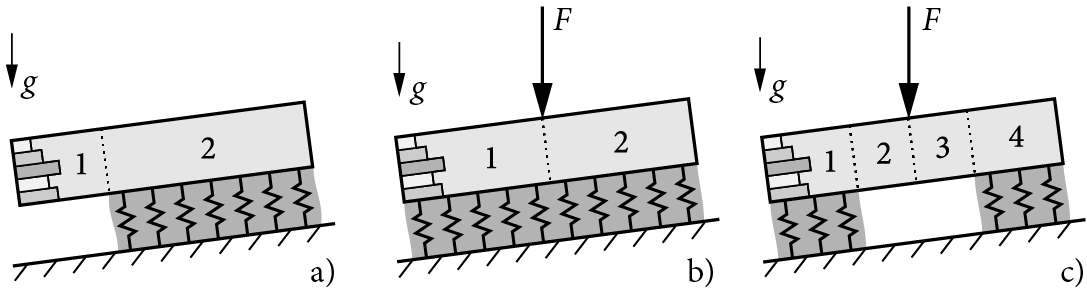
Read the 📄 white paper for model derivations, illustrations, dimensions, material properties, and kinematics:
Weißgraeber, P. & Rosendahl, P. L. (2023). A closed-form model for layered snow slabs. The Cryosphere, 17(4), 1475–1496. https://doi.org/10.5194/tc-17-1475-2023
For more background info, please refer to the companion papers:
Rosendahl, P. L. & Weißgraeber, P. (2020). Modeling snow slab avalanches caused by weak-layer failure – Part 1: Slabs on compliant and collapsible weak layers. The Cryosphere, 14(1), 115–130. https://doi.org/10.5194/tc-14-115-2020
Rosendahl, P. L. & Weißgraeber, P. (2020). Modeling snow slab avalanches caused by weak-layer failure – Part 2: Coupled mixed-mode criterion for skier-triggered anticracks. The Cryosphere, 14(1), 131–145. https://doi.org/10.5194/tc-14-131-2020
The following describes the basic usage of WEAC. Please refer to the demo for more examples and read the documentation for details.
Load the module.
importweac
Choose a snow profile from the preconfigured profiles (see dummy_profiles in demo) or create your own using the Layer Pydantic class. One row corresponds to one layer counted from top (below surface) to bottom (above weak layer).
Create a Scenario that defines the environment and setup that the slab and weak layer will be evaluated in.
fromweac.componentsimportScenarioConfig, Segment# Example 1: SKIERskier_config=ScenarioConfig(
system_type='skier',
phi=30,
)
skier_segments= [
Segment(length=5000, has_foundation=True, m=0),
Segment(length=0, has_foundation=False, m=80),
Segment(length=0, has_foundation=False, m=0),
Segment(length=5000, has_foundation=True, m=0),
] # Scenario is a skier of 80 kg standing on a 10 meter long slab at a 30 degree angle# Exampel 2: PSTpst_config=ScenarioConfig(
system_type='pst-', # Downslope cutphi=30, # (counterclockwise positive)cut_length=300,
)
pst_segments= [
Segment(length=5000, has_foundation=True, m=0),
Segment(length=300, has_foundation=False, m=0), # Crack Segment
] # Scenario is Downslope PST with a 300mm cut
Create a SystemModel instance that combines the inputs and handles system solving and field-quantity extraction.
fromweac.componentsimportConfig, ModelInputfromweac.core.system_modelimportSystemModel# Example: build a model for the skier scenario defined above model_input=ModelInput(
weak_layer=weak_layer,
scenario_config=skier_config,
layers=custom_layers,
segments=skier_segments,
)
system_config=Config(
touchdown=True
)
skier_system=SystemModel(
model_input=model_input,
config=system_config,
)
Unknown constants are cached_properties; calling skier_system.unknown_constants solves the system of linear equations and extracts the constants.
C=skier_system.unknown_constants
Analyzer handles rasterization + computation of involved slab and weak-layer properties Sxx, Sxz, etc.
Prepare the output by rasterizing the solution vector at all horizontal positions xsl (slab). The result is returned in the form of the ndarray z. We also get xwl (weak layer) that only contains x-coordinates that are supported by a foundation.
fromweac.analysis.analyzerimportAnalyzerskier_analyzer=Analyzer(skier_system)
xsl_skier, z_skier, xwl_skier=skier_analyzer.rasterize_solution(mode="cracked")
Gdif, GdifI, GdifII=skier_analyzer.differential_ERR()
Ginc, GincI, GincII=skier_analyzer.incremental_ERR()
# and Sxx, Sxz, Tzz, principal stress, incremental_potential, ...
Visualize the results.
fromweac.analysis.plotterimportPlotterplotter=Plotter()
# Visualize slab profilefig=plotter.plot_slab_profile(
weak_layers=weak_layer,
slabs=skier_system.slab,
)
# Visualize deformations as a contour plotfig=plotter.plot_deformed(
xsl_skier, xwl_skier, z_skier, skier_analyzer, scale=200, window=200, aspect=2, field="Sxx"
)
# Plot slab displacements (using x-coordinates of all segments, xsl)plotter.plot_displacements(skier_analyzer, x=xsl_skier, z=z_skier)
# Plot weak-layer stresses (using only x-coordinates of bedded segments, xwl)plotter.plot_stresses(skier_analyzer, x=xwl_skier, z=z_skier)
Compute output/field quantities for exporting or plotting.
# Compute stresses in kPa in the weaklayertau=skier_system.fq.tau(Z=z_skier, unit='kPa')
sig=skier_system.fq.sig(Z=z_skier, unit='kPa')
w=skier_system.fq.w(Z=z_skier, unit='um')
# Example evaluation vertical displacement at top/mid/bottom of the slabu_top=skier_system.fq.u(Z=z_skier, h0=top, unit='um')
u_mid=skier_system.fq.u(Z=z_skier, h0=mid, unit='um')
u_bot=skier_system.fq.u(Z=z_skier, h0=bot, unit='um')
psi=skier_system.fq.psi(Z=z_skier, unit='deg')
Roadmap
See the open issues for a list of proposed features and known issues.
v4.0
Change to scenario & scenario_config: InfEnd/Cut/Segment/Weight
v3.2
Complex terrain through the addition of out-of-plane tilt
Up, down, and cross-slope cracks
v3.1
Improved CriteriaEvaluator Optimization (x2 time reduction)
Release history
v3.0
Refactored the codebase for improved structure and maintainability
Added property caching for improved efficiency
Added input validation
Adopted a new, modular, and object-oriented design
v2.6
Introduced test suite
Mitraged from setup.cfg to pyproject.toml
Added parametrization for collaps heights
v2.5
Analyze slab touchdown in PST experiments by setting touchdown=True
Completely redesigned and significantly improved API documentation
v2.4
Choose between slope-normal ('-pst', 'pst-') or vertical ('-vpst', 'vpst-') PST boundary conditions
v2.3
Stress plots on deformed contours
PSTs now account for slab touchdown
v2.2
Sign of inclination phi consistent with the coordinate system (positive counterclockwise)
Dimension arguments to field-quantity methods added
Improved aspect ratio of profile views and contour plots
Improved plot labels
Convenience methods for the export of weak-layer stresses and slab deformations provided
Wrapper for (re)calculation of the fundamental system added
Now allows for distributed surface loads
v2.1
Consistent use of coordinate system with downward pointing z-axis
Consitent top-to-bottom numbering of slab layers
Implementation of PSTs cut from either left or right side
v2.0
Completely rewritten in 🐍 Python
Coupled bending-extension ODE solver implemented
Stress analysis of arbitrarily layered snow slabs
FEM validation of
displacements
weak-layer stresses
energy release rates in weak layers
Documentation
Demo and examples
v1.0
Written in 🌋 MATLAB
Deformation analysis of homogeneous snow labs
Weak-layer stress prediction
Energy release rates of cracks in weak layers
Finite fracture mechanics implementation
Prediction of anticrack nucleation
How to contribute
Fork the project
Initialize submodules
git submodule update --init --recursive
Create your feature branch (git checkout -b feature/amazingfeature)
Commit your changes (git commit -m 'Add some amazing feature')
Push to the branch (git push origin feature/amazingfeature)
Share — copy and redistribute the material in any medium or format
Adapt — remix, transform, and build upon the material for any purpose, even commercially.
Under the following terms:
Attribution — You must give appropriate credit, provide a link to the license, and indicate if changes were made. You may do so in any reasonable manner, but not in any way that suggests the licensor endorses you or your use.
Rosendahl, P. L., Schneider, J., & Weissgraeber, P. (2022). Weak Layer Anticrack Nucleation Model (WEAC). Zenodo. https://doi.org/10.5281/zenodo.5773113
Read the 📄 white paper for model derivations, illustrations, dimensions, material properties, and kinematics:
Weißgraeber, P. & Rosendahl, P. L. (2023). A closed-form model for layered snow slabs. The Cryosphere, 17(4), 1475–1496. https://doi.org/10.5194/tc-17-1475-2023
For more background info, please refer to the companion papers:
Rosendahl, P. L. & Weißgraeber, P. (2020). Modeling snow slab avalanches caused by weak-layer failure – Part 1: Slabs on compliant and collapsible weak layers. The Cryosphere, 14(1), 115–130. https://doi.org/10.5194/tc-14-115-2020
Rosendahl, P. L. & Weißgraeber, P. (2020). Modeling snow slab avalanches caused by weak-layer failure – Part 2: Coupled mixed-mode criterion for skier-triggered anticracks. The Cryosphere, 14(1), 131–145. https://doi.org/10.5194/tc-14-131-2020
The following describes the basic usage of WEAC. Please refer to the demo for more examples and read the documentation for details.
Load the module.
importweac
Choose a snow profile from the preconfigured profiles (see dummy_profiles in demo) or create your own using the Layer Pydantic class. One row corresponds to one layer counted from top (below surface) to bottom (above weak layer).
Create a Scenario that defines the environment and setup that the slab and weak layer will be evaluated in.
fromweac.componentsimportScenarioConfig, Segment# Example 1: SKIERskier_config=ScenarioConfig(
system_type='skier',
phi=30,
)
skier_segments= [
Segment(length=5000, has_foundation=True, m=0),
Segment(length=0, has_foundation=False, m=80),
Segment(length=0, has_foundation=False, m=0),
Segment(length=5000, has_foundation=True, m=0),
] # Scenario is a skier of 80 kg standing on a 10 meter long slab at a 30 degree angle# Exampel 2: PSTpst_config=ScenarioConfig(
system_type='pst-', # Downslope cutphi=30, # (counterclockwise positive)cut_length=300,
)
pst_segments= [
Segment(length=5000, has_foundation=True, m=0),
Segment(length=300, has_foundation=False, m=0), # Crack Segment
] # Scenario is Downslope PST with a 300mm cut
Create a SystemModel instance that combines the inputs and handles system solving and field-quantity extraction.
fromweac.componentsimportConfig, ModelInputfromweac.core.system_modelimportSystemModel# Example: build a model for the skier scenario defined above model_input=ModelInput(
weak_layer=weak_layer,
scenario_config=skier_config,
layers=custom_layers,
segments=skier_segments,
)
system_config=Config(
touchdown=True
)
skier_system=SystemModel(
model_input=model_input,
config=system_config,
)
Unknown constants are cached_properties; calling skier_system.unknown_constants solves the system of linear equations and extracts the constants.
C=skier_system.unknown_constants
Analyzer handles rasterization + computation of involved slab and weak-layer properties Sxx, Sxz, etc.
Prepare the output by rasterizing the solution vector at all horizontal positions xsl (slab). The result is returned in the form of the ndarray z. We also get xwl (weak layer) that only contains x-coordinates that are supported by a foundation.
fromweac.analysis.analyzerimportAnalyzerskier_analyzer=Analyzer(skier_system)
xsl_skier, z_skier, xwl_skier=skier_analyzer.rasterize_solution(mode="cracked")
Gdif, GdifI, GdifII=skier_analyzer.differential_ERR()
Ginc, GincI, GincII=skier_analyzer.incremental_ERR()
# and Sxx, Sxz, Tzz, principal stress, incremental_potential, ...
Visualize the results.
fromweac.analysis.plotterimportPlotterplotter=Plotter()
# Visualize slab profilefig=plotter.plot_slab_profile(
weak_layers=weak_layer,
slabs=skier_system.slab,
)
# Visualize deformations as a contour plotfig=plotter.plot_deformed(
xsl_skier, xwl_skier, z_skier, skier_analyzer, scale=200, window=200, aspect=2, field="Sxx"
)
# Plot slab displacements (using x-coordinates of all segments, xsl)plotter.plot_displacements(skier_analyzer, x=xsl_skier, z=z_skier)
# Plot weak-layer stresses (using only x-coordinates of bedded segments, xwl)plotter.plot_stresses(skier_analyzer, x=xwl_skier, z=z_skier)
Compute output/field quantities for exporting or plotting.
# Compute stresses in kPa in the weaklayertau=skier_system.fq.tau(Z=z_skier, unit='kPa')
sig=skier_system.fq.sig(Z=z_skier, unit='kPa')
w=skier_system.fq.w(Z=z_skier, unit='um')
# Example evaluation vertical displacement at top/mid/bottom of the slabu_top=skier_system.fq.u(Z=z_skier, h0=top, unit='um')
u_mid=skier_system.fq.u(Z=z_skier, h0=mid, unit='um')
u_bot=skier_system.fq.u(Z=z_skier, h0=bot, unit='um')
psi=skier_system.fq.psi(Z=z_skier, unit='deg')
Roadmap
See the open issues for a list of proposed features and known issues.
v4.0
Change to scenario & scenario_config: InfEnd/Cut/Segment/Weight
v3.2
Complex terrain through the addition of out-of-plane tilt
Up, down, and cross-slope cracks
v3.1
Improved CriteriaEvaluator Optimization (x2 time reduction)
Release history
v3.0
Refactored the codebase for improved structure and maintainability
Added property caching for improved efficiency
Added input validation
Adopted a new, modular, and object-oriented design
v2.6
Introduced test suite
Mitraged from setup.cfg to pyproject.toml
Added parametrization for collaps heights
v2.5
Analyze slab touchdown in PST experiments by setting touchdown=True
Completely redesigned and significantly improved API documentation
v2.4
Choose between slope-normal ('-pst', 'pst-') or vertical ('-vpst', 'vpst-') PST boundary conditions
v2.3
Stress plots on deformed contours
PSTs now account for slab touchdown
v2.2
Sign of inclination phi consistent with the coordinate system (positive counterclockwise)
Dimension arguments to field-quantity methods added
Improved aspect ratio of profile views and contour plots
Improved plot labels
Convenience methods for the export of weak-layer stresses and slab deformations provided
Wrapper for (re)calculation of the fundamental system added
Now allows for distributed surface loads
v2.1
Consistent use of coordinate system with downward pointing z-axis
Consitent top-to-bottom numbering of slab layers
Implementation of PSTs cut from either left or right side
v2.0
Completely rewritten in 🐍 Python
Coupled bending-extension ODE solver implemented
Stress analysis of arbitrarily layered snow slabs
FEM validation of
displacements
weak-layer stresses
energy release rates in weak layers
Documentation
Demo and examples
v1.0
Written in 🌋 MATLAB
Deformation analysis of homogeneous snow labs
Weak-layer stress prediction
Energy release rates of cracks in weak layers
Finite fracture mechanics implementation
Prediction of anticrack nucleation
How to contribute
Fork the project
Initialize submodules
git submodule update --init --recursive
Create your feature branch (git checkout -b feature/amazingfeature)
Commit your changes (git commit -m 'Add some amazing feature')
Push to the branch (git push origin feature/amazingfeature)
Share — copy and redistribute the material in any medium or format
Adapt — remix, transform, and build upon the material for any purpose, even commercially.
Under the following terms:
Attribution — You must give appropriate credit, provide a link to the license, and indicate if changes were made. You may do so in any reasonable manner, but not in any way that suggests the licensor endorses you or your use.
This is a rewrite version of discord-modmail due to the breaking changes released by Discord where all bots are expected to migrate over to Slash Commands by April 2022. Discord ticketing serves as a shared inbox for server moderators to communicate with users in a seamless way via a ticketing system.
How does it work?
User is able to raise a ticket by interacting with the buttons on a support message which consists of various support categories configured by the server. A subsequent text channel will be created between both the user and support staffs that has the corresponding role belonging to the support category.
Commands Usage
Server Administrators
/setup – Automatically sets up the ticketing module in the server
/disable – Close all current threads and disable ticketing
/react – Sends a message that listens for interactions with the buttons
/create_flag <name> <points> – Create a claimable flag with the specified points
/delete_flag <name> – Delete previously created flag
/create_role <name> <emoji> – Create a role with the specified emoji that will be displayed as a button on the main ticketing message
/delete_role <name> – Delete previously created role that appears on ticketing message
/add_regex <regexPattern>– Add a regex pattern in memory for bot to watch for blacklisted messages
/enable_cog <cog> – Manually enable a cog
/disable_cog <cog> – Manually disable a cog
Moderators
/block <user> – Blocks specified user and prevent them from utilising ticketing system
/unblock <user> – Unblocks specified user
Sponsors
/add <user> [points] – Awards point(s) (default = 1) to specified user
/minus <user> [points] – Deducts point(s) (default = 1) from specified user
Users
/list – Display user points according to the points awarded by various flags and sponsors
/flag <name> – Submit a flag and earn points
Notes
Moderators must be assigned a support role (specified in environment variables) to access the commands.
Sponsors commands are a requested feature for a specific use case. @Sponsor roles are required to access these commands.
This repository is built on base-template of Pytorch Template which is bi-product of original Pytorch Project Template. Check the template repositories first before getting started.
The main difference from Show, Attend and Tell is that I replaced row-encoder to positional encoding. And I set less ‘max sequence length’ with 40. With these changes, I could get perplexity of 1.0717 with reliable performance.
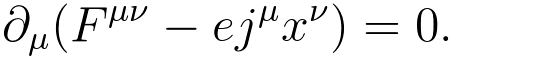
im2latex Result = \partial _ { \mu } ( F ^ { \mu \nu } - e j ^ { \mu } x ^ { \nu } ) : 0 .
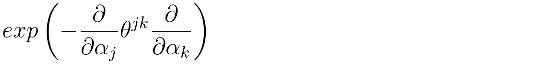
im2latex Result : e x p \left( - \frac { \partial } { \partial \alpha _ { j } } \theta ^ { i k } \frac { \partial } { \partial \alpha _ { k } } \right)
He provides his data processing strategy, so you can follow his preprocessing steps.
If you are in hurry, you can just download Full Dataset as well.
Then you will have Ascii-LaTeX Formula Text Datasets around 140K formulas. Though you can get full formula images from untrix’s dataset, I recommend to render the image yourself with LaTeX text dataset.
You can use sympy library to render formula from LaTeX text. With data/custom_preprocess_v2.py, you can render two type of formula image with Euler font deciding variable.
2. Edit json configs file
If your data path is different, edit configs/draft.json.
This repository is built on base-template of Pytorch Template which is bi-product of original Pytorch Project Template. Check the template repositories first before getting started.
The main difference from Show, Attend and Tell is that I replaced row-encoder to positional encoding. And I set less ‘max sequence length’ with 40. With these changes, I could get perplexity of 1.0717 with reliable performance.
im2latex Result = \partial _ { \mu } ( F ^ { \mu \nu } - e j ^ { \mu } x ^ { \nu } ) : 0 .
im2latex Result : e x p \left( - \frac { \partial } { \partial \alpha _ { j } } \theta ^ { i k } \frac { \partial } { \partial \alpha _ { k } } \right)
He provides his data processing strategy, so you can follow his preprocessing steps.
If you are in hurry, you can just download Full Dataset as well.
Then you will have Ascii-LaTeX Formula Text Datasets around 140K formulas. Though you can get full formula images from untrix’s dataset, I recommend to render the image yourself with LaTeX text dataset.
You can use sympy library to render formula from LaTeX text. With data/custom_preprocess_v2.py, you can render two type of formula image with Euler font deciding variable.
2. Edit json configs file
If your data path is different, edit configs/draft.json.
Tento repozitár je určený pre výučbu predmetu B-VSA vyučovaný na FEI STU Bratislava počas letného semestra 2021/2022.
Jednotlivé branches repozitáru demonštrujú problematiku preberanú na jednotlivých cvičeniach.
Cieľom cvičenia 11 je ukážka definovanie REST špecifikácie pomocou štandardu OpenAPI3 (viď
súbor b-vsa-openapi.yml) a demonštrovať implementáciu REST webových služieb
pomocou JAX-RS (framework jersey), nastavenia aplikačného servera a testovanie HTTP požiadavok.
Projekt taktiež zahŕňa ukážku práce s HTTP hlavičkami a autentifikáciou používateľa cez Basic Auth.
Pre demonštráciu problematiky cvičenie využíva databázu MySQL a JPA implementáciu EclipseLink, Jersey a HTTP server
Grizzly2. Jednotlivé triedy aplikácie slúžia výhradne na demonštráciu problematiky.
Inštalácia a spustenie
Cvičenie je implementované, ako Maven projekt
pre Java 1.8. Nakoľko cvičenie demonštruje prácu s databázou je potrebné mať
nainštalovanú databázu MySQL 5.7+.
Nastavenie projektu
Projekt je možné otvoriť v ľubovolnom modernom IDE (testované na IntelliJ Idea a Visual Studio Code), podporujúci Maven
projekt manažment.
Pre kompiláciu projektu do JAR archívu je možné použiť príkaz:
mvn clean package verify
Vytvorenie databázy
Pre správne otestovanie funkcionality aplikácie je potrebné mať nainštalovanú databázy MySQL vo verzií 5.7 a vyššie. Po
spustení databázové servera je potrebné vytvoriť databázu a používateľ pre potreby aplikácie.
Názov databázy a prihlasovacie údaje používateľa musia byť totožné s uvedenými v
súbor persistence.xml. Uvedený SQL skript pracuje s defaultnými
hodnotami.
CREATEDATABASEIF NOT EXISTS VSA_CV11 CHARACTER SET utf8mb4 COLLATE utf8mb4_unicode_ci;
CREATEUSERIF NOT EXISTS 'vsa'@'localhost' IDENTIFIED BY 'vsa';
GRANT ALL PRIVILEGES ON VSA_CV11.* TO 'vsa'@'localhost';
FLUSH PRIVILEGES;
HANDY is interactive Python3 program for spectrum normalization. The normalization process is based on “regions” and “ranges”. “Ranges” are continuum parts defined manually by user (or uploaded from file from previous program run) which will be used for continuum level fit. “Regions” are groups of ranges for whom single chebyshev polynomial of chosen order is fitted. Polynomial fits are connected with the use of Akima’a spline interpolation. The program offers graphical access to theoretical grid of spectra for obtaining an idea about processed star atmosphere parameters and interface for radial velocity correction. Different grids of spectra can be easly added by the user.
Interactive normalization of spectrum in single run
Portability of continuum ranges between different spectra
Easy access to precomputed grid of NLTE stars spectra (computed with SYNSPEC, with use of BSTAR2006 models)
NLTE line blanketed model atmospheres of hot stars. I. Hybrid Complete Linearization/Accelerated Lambda Iteration Method, 1995, Hubeny, I., & Lanz, T., Astrophysical Journal, 439, 875
Easy access to ATLAS/SYNTHE (Kurucz,R.L., 1993) code via VidmaPy package. Used precompiled codes and works only under Linux.
Adding user defined grids
Radial velocity correction
Developed and tested on Linux
Easy installation and easy to use
Getting Started
Prerequisites
Python3
Conda – recommended but not necessary
Download
Two steps:
Clone the repository or download it as the .zip file:
Now you have to clone submodule VidmaPy by calling (from HANDY catalogue):
git submodule update --init
It should clone the vidmapy in to HANDY/vidmapy. The next step is the installation of VidmaPy that enable HANDY to use ATLAS/SYNTHE. To install the vidmapy in HANDY-env environment (you want that), you need to follow the description from VidmaPy README.
Shortly speaking:
download atomic data and place in directory (three distinct directories: ODF, molecules, and lines):
After that you may want to make symbolic link in your ~/bin/ directory to HANDY.sh file to be able to easly run the program in whole system. Eg. on my system:
ln -s ~/repos/HANDY/HANDY.sh ~/bin/HANDY
Then you should be able to simply run the program by executing:
HANDY
in your terminal.
Update
If you used git to install HANDY you can easy update HANDY just by pulling changes from remote:
git pull
Otherwise you need to re-install HANDY from newly downloaded .zip file.
Tutorial
Full description and tutorial could be find in HANDY project GitHub page:


 https://github.com/tamada/gixor